Introduction: Why Care DCT?
We have been using Discrete Cosine Transform (DCT) without possibly awaring of it: DCT is actually the JPEG compression standard!
In audio analysis, DCT is used in computing MFCC coefficients to extract feature vector (for more on MFCCs, see [KC] in reference section), which makes deep learning on sound possible by
-
Treating the sequence of MFCC coefficients as a time sequence of data (at each "window" of suitable "hop length", we get a float vector of fixed size) or;
-
Stacking the MFCC coefficients and treat it as an image.
In the former case the use of sequence model such as LSTM or Transformer becomes possible. The later case makes it possible to use convolution layer such as Conv1D in Keras.
Basic Knowledge to Work With
Definitions
In what follows for we will denote
For each fixed we will consider as a function on a discrete domain. The vectors
form an orthonormal basis in , by stacking all them together column by column
then is orthonormal: .
The orthogonality of and the construction of the basis will be explained in Mathematics behind DCT section. For now let's enjoy the coding and see the results.
Computations
We make explicit calculations in order to make readers comfortable with the definition above.
First, given a gray-scale image there are always unique coefficients such that
In fact by using defined in the previous section. Denote also as the matrix with entry at -th row and -th column, if we define , then
You can expand the RHS () to convince yourself that eventually you get the same expression as in . On the other hand, by using this we have the reverse:
as this is not a summation of 's of fixed frequencies, that's why we don't define .
Our coding will strictly follow the notation and calculation in this section.
Implementation of JPEG Compression in Python
For readers who are more familiar with matlab, you may also follow the youtube video listed in [ET]. Most of the content is a translation from matlab to python based on my understanding.
Notation and definition may be different from the video.
Basic Import
import numpy as np import matplotlib.pyplot as plt from tensorflow.keras.preprocessing.image import img_to_array, load_img %matplotlib inline
Constants
N = 8 IMAGE_PATH = "512_512_image.jpg"
Basis of Cosine Transform
def range2D(n): indexes = [] for i in range(0, n): for j in range(0, n): indexes.append((i, j)) return indexes def alpha(p): return 1/np.sqrt(N) if p == 0 else np.sqrt(2/N) def cos_basis(i,j): def cal_result(a): x=a[0] y=a[1] return alpha(i) * alpha(j) * np.cos((2*x+1) * i * np.pi/(2*N)) * np.cos((2*y+1) * j * np.pi/(2*N)) return cal_result
Plot of the 2D Cosine Basis Functions
fig = plt.figure() fig.set_figheight(12) fig.set_figwidth(12) xy_range = range2D(N) xy_plane_NxN = (np.array(xy_range).reshape(N,N,2)) for i in range(0, N): for j in range(0, N): xy_result = np.apply_along_axis(cos_basis(i,j), -1, xy_plane_NxN) plt.subplot(N, N, 1 + N*i + j) plt.imshow(xy_result, cmap="gray")

Compute Coefficients for Cosine Transform
Let's prepare the following matrix that convert the original pixels into compacted energy distribution:
U = np.zeros((N,N)) for i in range(0, N): for j in range(0, N): U[i, j] = alpha(j) * np.cos((2*i+1)*j*np.pi/(2*N)) U_t = U.transpose()
You may check that U is indeed orthonormal by:
np.matmul(U, U_t) # Result: # array([[ 1.00000000e+00, -1.01506949e-16, -3.78598224e-17, # -1.03614850e-17, -1.33831237e-16, 7.88118312e-17, # 2.00856868e-16, -1.70562493e-16], # [-1.01506949e-16, 1.00000000e+00, 1.70298111e-17, # -1.13980777e-17, 1.37840552e-16, -2.88419699e-16, # -1.24636773e-16, 2.51800326e-17], # [-3.78598224e-17, 1.70298111e-17, 1.00000000e+00, # -1.61419161e-16, -2.81922100e-17, -1.25319880e-16, # -1.83252893e-16, -2.79432802e-17], # [-1.03614850e-17, -1.13980777e-17, -1.61419161e-16, # 1.00000000e+00, -1.92659768e-17, 2.75108042e-16, # 2.02487213e-16, 2.22263103e-18], # [-1.33831237e-16, 1.37840552e-16, -2.81922100e-17, # -1.92659768e-17, 1.00000000e+00, -8.54966705e-17, # -2.36183557e-17, -3.71508058e-16], # [ 7.88118312e-17, -2.88419699e-16, -1.25319880e-16, # 2.75108042e-16, -8.54966705e-17, 1.00000000e+00, # 1.21575873e-16, 8.41357861e-17], # [ 2.00856868e-16, -1.24636773e-16, -1.83252893e-16, # 2.02487213e-16, -2.36183557e-17, 1.21575873e-16, # 1.00000000e+00, 3.92417644e-16], # [-1.70562493e-16, 2.51800326e-17, -2.79432802e-17, # 2.22263103e-18, -3.71508058e-16, 8.41357861e-17, # 3.92417644e-16, 1.00000000e+00]])
Mask or Truncate the Energy Distribution
Here we use a naive approach, we screen out the fourier coefficents by simply retaining those from the upper-left corner. For that, we create a mask:
def create_mask(closure): mask = np.zeros((N, N)) for i in range(N): for j in range(N): if closure(i,j): mask[i, j] = 1 return mask
For example, by calling mask = create_mask(lambda i,j: 0<=i+j<=2) our mask will be like:
[[1. 1. 1. 0. 0. 0. 0. 0.] [1. 1. 0. 0. 0. 0. 0. 0.] [1. 0. 0. 0. 0. 0. 0. 0.] [0. 0. 0. 0. 0. 0. 0. 0.] [0. 0. 0. 0. 0. 0. 0. 0.] [0. 0. 0. 0. 0. 0. 0. 0.] [0. 0. 0. 0. 0. 0. 0. 0.] [0. 0. 0. 0. 0. 0. 0. 0.]]
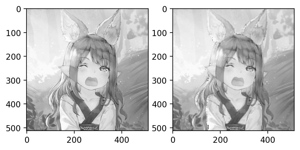
Result: Apply Cosine Transform
original = load_img(IMAGE_PATH, target_size=(512, 512), color_mode="grayscale") original = img_to_array(original).astype("uint8") original = np.squeeze(original) original.shape mask = create_mask(lambda i,j: 0<=i+j<=2) print(mask) steps = int(original.shape[0]/N) # we choose 512x512 image, therefore steps = 64 print(steps) compressed = np.zeros_like(original) for x in range(steps): for y in range(steps): sub_pixels = original[N * y: N*(y+1), N * x: N*(x+1)] sub_pixels = sub_pixels - 127.5 fourier_coefficients = np.matmul(np.matmul(U_t, sub_pixels), U) fourier_coefficients = fourier_coefficients * mask reverted_pixels = np.matmul(np.matmul(U, fourier_coefficients), U_t) reverted_pixels = reverted_pixels + 127.5 compressed[N * y: N*(y+1), N * x: N*(x+1)] = reverted_pixels fig.set_figheight(20) fig.set_figwidth(20) plt.subplot(1, 2, 1) plt.imshow(original, cmap="gray") plt.subplot(1, 2, 2) plt.imshow(compressed, cmap="gray") plt.savefig("DCT_result", dpi=200, bbox_inches="tight")
Mathematics behind DCT
Notation. Every vector will be considered as a column vector whenever the computation does not make sense when they are represented as a row.
From DFT
Let be an integer and denote , define then the matrix
is orthogonal simply because their inner product
is when , where . Therefore the basis forms an orthogonal basis in .
But how to find a similar basis in ? It is not as simple as taking the real part of the linear combination since the coordinate even .
DCT-2
Strategy of Construction
Consider the symmetric second difference matrix:
which arises when a second derivate is approximated by the central second difference:
as .
Let denote the values of a function evaluated on the discretized domain of , i.e., for some , where : means stacking values by running through all indexes at that position.
Our cosine transform is based on decomposing a function into a linear combination of cosine functions (of different frequencies) in discrete case. To find them, we will choose such that . By the fact that:
Fact. Eigenvectors associated to different eigenvalues are linearly independent.
we then obtain a set of eigenvectors (of different eigenvalues) solving the approximated problem
Which function would solve the ODE ? Which is the trigonometric function!
Why and ?
These two assignments are determined by imposing boundary conditions. More specific, we extend the domain from to , imagine we are solving (append one point at the beginning and the tail of respectively).
We have not imposed any boundary condition to our solution yet. We will require our function be symmetric at (or at if , ), this implies .
At another boundary due to the shift above, we try to require , this implies .
and plug this condition into the second difference formula to get:
These become the necessary condition and thus have determined our and , and therefore ensure our solution is a cosine function.
Different values of 's and 's will correspond to different boundary condition imposed on for other combinations, see [GS] for a complete classification.
The solution corresponding to and is usally called the basis of DCT-2 (or simply DCT).
Derivation of the Basis of Discrete Cosine Transform
We have spent many effort to determine the matrix to work with, let's start with computing the basis directly for our only candidate:
Let for some , denote
note that we have whenever for integer . As we will see this is indeed the case later for .
Since , then for , coordinate-wise:
Therefore for whatever linear we choose (here ).
By taking real part on both sides, as is real, we have
here denotes the standard basis in . It remains to require satisfies and , from which we can determine and thus .
The equation implies , since is even, it is sufficient to require
The equation implies
for this to hold, it is sufficient to require (as is always symmetric about for every ), altogether we have , and thus for ,
Finally, we have
for suitably chosen 's, .
Reference
-
[KC] Kartik Chaudhary, Understanding Audio data, Fourier Transform, FFT and Spectrogram features for a Speech Recognition System,
-
[GS] Gilbert Strang, The Discrete Cosine Transform
-
[ET] Exploring Technologies, Discrete Cosine Transform (DCT) of Images and Image Compression