Result on Local Machine
Due to time constraint I didn't wait the model to train for long enough time as It is convincing to me that the model is trying to converge.
Reference
Main reference for coding part:
Other references for theory:
- Denoising Diffusion Probabilitic Model
- Diffusion Model:比“GAN"还要牛逼的图像生成模型!公式推导+论文精读,迪哥打你从零详解扩散模型!
- Stable Diffusion: High-Resolution Image Synthesis with Latent Diffusion Models | ML Coding Series
Introduction
-
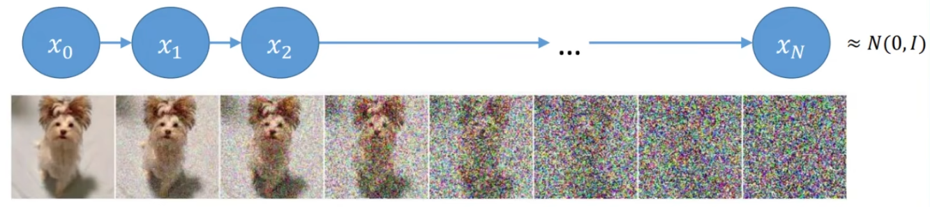
Define as the image at time for . When we travel about , we add noise gradually until the image is unreadable. The noise is added by
for , where and .
-
In practice (coding) will go from to , needs not be very small when the noise is enough.
-
Note that started from , we no longer consider as a concrete image, rather we consider as a random variable where only the mean and variance makes perfect sense.
-
The true image depense on the instance of values that a gaussian noise provide.
-
That means denotes a set of possibilities of images (data point). To understant , we need to understand the density of the probability distribution .
-
By direct expansion we have
where .
-
Since , the last term becomes
for some .
-
Define for , then for some .
-
Note that .
-
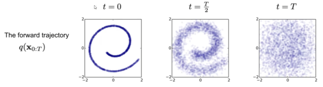
The forward process of adding noise is denoted
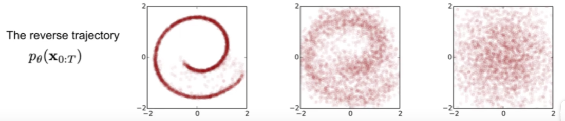
We wish to calculate the reverse (denoise) process
-
Recall the Bayse Forumla .
-
Given a set of images , we wish to understand the distribution of , i.e., we wish to calculate
-
usually is used to denote known distribution.
-
To emphasize we don't truly understand the distribution, we replace by to denote unknown distribution (the distribution that we are going to find or estimate, or to learn), the problem becomes estimating the distribution .
-
As we know we add random noise from to , it makes no sense to estimate the exact value of a random variable from .
-
Therefore what we want to estiamte is the average of from an instance of .
-
By Bayse formula, .
-
To enable ourself to do computation, we also assume follows Gaussian distribution.
-
We now try to estimate the mean of , name it .
-
We have already studied the distribution of in .
-
Suppose that is given and we know that it comes from the previous distribution by adding gaussian noise with some weight (in the same way as before), then
where .
-
By comparing coefficients we have
by we have
-
will be what we are trying to learn.
-
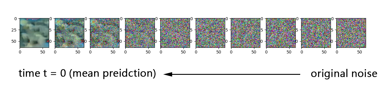
When we predict image in reverse timesteps, we iteratively predict image by
for some sampled from normal distribution. In code it is implemented as follows:
@torch.no_grad() def sample_timestep(model, x, t): """ Calls the model to predict the noise in the image and returns the denoised image. Applies noise to this image, if we are not in the last step yet. """ betas_t = get_index_from_list(betas, t, x.shape) sqrt_one_minus_alphas_cumprod_t = get_index_from_list( sqrt_one_minus_alphas_cumprod, t, x.shape ) sqrt_recip_alphas_t = get_index_from_list(sqrt_recip_alphas, t, x.shape) # Call model (current image - noise prediction) model_mean = sqrt_recip_alphas_t * ( x - betas_t * model(x, t) / sqrt_one_minus_alphas_cumprod_t ) posterior_variance_t = get_index_from_list(posterior_variance, t, x.shape) if t == 0: return model_mean else: noise = torch.randn_like(x) return model_mean + torch.sqrt(posterior_variance_t) * noise -
From to we add a noize . We estimate (learn) from to , then will be our ground truth in the model. We elaborate this in the next section.
In code it is implemented as follows:
def get_loss(model, x_0, times): # times is of shape (128, ) x_noisy, noise = forward_diffusion_sample(x_0, times, device) # 128 time times, therefore 128 images, x_noisy is of shape [128, 3, 64, 64] noise_pred = model(x_noisy, times) return F.l1_loss(noise, noise_pred)
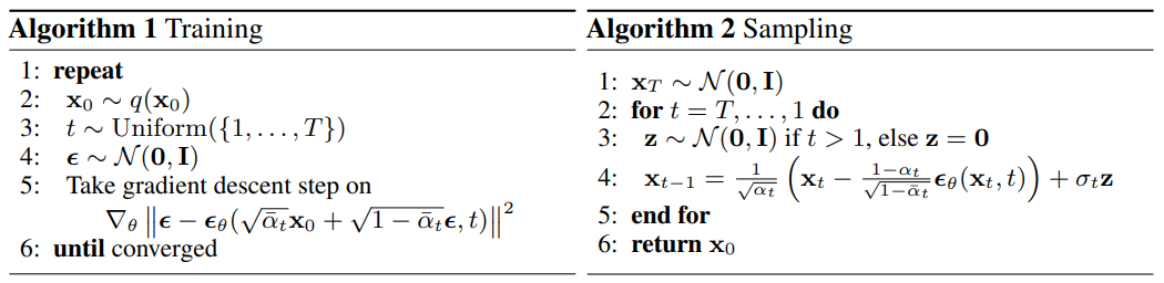
Training Algorithm
-
-
In algorithm on the LHS:
-
means we sample an image from our collection of image dataset ( means the distribution of the images that lives in, like category of dogs, cats, etc)
-
means the timestamp is uniformly random
-
means the noise we add from to .
-
is the estimate of from to (as we want to do the reverse). This is estimated from
- (see ) and
- timestamp
our loss function becomes .
-
Coding
Constants
def linear_beta_schedule(timesteps, start=0.0001, end=0.02): return torch.linspace(start, end, timesteps) def get_index_from_list(vals, t, x_shape): """ Returns a specific index t of a passed list of values vals while considering the batch dimension. """ batch_size = t.shape[0] out = vals.gather(-1, t.cpu()) # same as .reshape( (batch_size,) + ((1,) * (len(x_shape) - 1)) ) result = out.reshape(batch_size, *((1,) * (len(x_shape) - 1))).to(t.device) return result # Define beta schedule T = 300 IMG_SIZE = 64 TIMESTEPS_BATCH_SIZE = 128 betas = linear_beta_schedule(timesteps=T) # Pre-calculate different terms for closed form alphas = 1. - betas alphas_cumprod = torch.cumprod(alphas, axis=0) alphas_cumprod_prev = F.pad(alphas_cumprod[:-1], (1, 0), value=1.0) sqrt_recip_alphas = torch.sqrt(1.0 / alphas) sqrt_alphas_cumprod = torch.sqrt(alphas_cumprod) sqrt_one_minus_alphas_cumprod = torch.sqrt(1. - alphas_cumprod) posterior_variance = betas * (1. - alphas_cumprod_prev) / (1. - alphas_cumprod)
SinusoidalPositionEmbeddings
This is exactly the same as the one we use in transformer, which basically takes a time to a vector of size (32,).
To recall, positional encoding takes the following form: for each fixed ,
where .
1class SinusoidalPositionEmbeddings(nn.Module):
2    def __init__(self, dim):
3        super().__init__()
4        # dim = 32
5        self.dim = dim
6
7    def forward(self, times):
8        half_dim = self.dim // 2
9        embeddings = math.log(10000) / (half_dim - 1)
10        embeddings = torch.exp(torch.arange(half_dim, device=device) * -embeddings)
11
12        # a_i = 1/10000^(i/half_dim)
13        # embeddings above = [a_1, a_2, a_3, ..., a_16]
14        embeddings = times[:, None] * embeddings[None, :]
15        # embeddings above <=>
16        # t |-> ( sin t*a_1, cos t*a_1, sin t*a_2, cos t*a_2, sin t*a_3, cos t*a_3, ... )
17        # for each t, therefore the final dimension will be (128, 32)
18        embeddings = torch.cat((embeddings.sin(), embeddings.cos()), dim=-1)
19        # TODO: Double check the ordering here
20        return embeddings
The variable embeddings in line 14 above is exactly
with timestep in place of pos above.
UNet that Predicts Noise
class SimpleUnet(nn.Module): """ A simplified variant of the Unet architecture. """ def __init__(self): super().__init__() image_channels = 3 down_channels = (64, 128, 256, 512, 1024) up_channels = (1024, 512, 256, 128, 64) out_dim = 1 time_emb_dim = 32 # Time embedding self.time_mlp = nn.Sequential( SinusoidalPositionEmbeddings(time_emb_dim), nn.Linear(time_emb_dim, time_emb_dim), nn.ReLU() ).to(device) # Initial projection # stride = 1, padding = 1, no change in spatial dimension self.conv0 = nn.Conv2d(image_channels, down_channels[0], 3, padding=1).to(device) # Downsample self.downs = nn.ModuleList([Block(down_channels[i], down_channels[i + 1], time_emb_dim).to(device) for i in range(len(down_channels) - 1)]) # Upsample self.ups = nn.ModuleList([Block(up_channels[i], up_channels[i + 1], time_emb_dim, up=True).to(device) for i in range(len(up_channels) - 1)]) self.output = nn.Conv2d(up_channels[-1], 3, out_dim).to(device) def forward(self, x, times): # Embedd time t = self.time_mlp(times) # Initial conv x = self.conv0(x) # Unet residual_inputs = [] for down in self.downs: x = down(x, t) residual_inputs.append(x) for up in self.ups: # for the bottom block the x adds an identical copy of x (just poped out) for unity of coding. residual_x = residual_inputs.pop() # Add residual x as additional channels x = torch.cat((x, residual_x), dim=1) x = up(x, t) return self.output(x)
Sampling / Prediction
@torch.no_grad() def sample_timestep(model, x, t): """ Calls the model to predict the noise in the image and returns the denoised image. Applies noise to this image, if we are not in the last step yet. """ betas_t = get_index_from_list(betas, t, x.shape) sqrt_one_minus_alphas_cumprod_t = get_index_from_list( sqrt_one_minus_alphas_cumprod, t, x.shape ) sqrt_recip_alphas_t = get_index_from_list(sqrt_recip_alphas, t, x.shape) # Call model (current image - noise prediction) model_mean = sqrt_recip_alphas_t * ( x - betas_t * model(x, t) / sqrt_one_minus_alphas_cumprod_t ) posterior_variance_t = get_index_from_list(posterior_variance, t, x.shape) if t == 0: return model_mean else: noise = torch.randn_like(x) return model_mean + torch.sqrt(posterior_variance_t) * noise @torch.no_grad() def sample_plot_image(model, img_path): # Sample noise img_size = IMG_SIZE img = torch.randn((1, 3, img_size, img_size), device=device) plt.figure(figsize=(15, 15)) plt.axis('off') num_images = 10 stepsize = int(T / num_images) for i in range(0, T)[::-1]: # just create a tensor t of shape (1,), the result is [1], [2], ..., etc times = torch.full((1,), i, device=device, dtype=torch.long) img = sample_timestep(model, img, times) if i % stepsize == 0: plt.subplot(1, num_images, i // stepsize + 1) show_tensor_image(img.detach().cpu()) plt.savefig(img_path)