tf.data.Dataset
Storing a set of images require a lot of memory, but saving a list of strings does not. In tensorflow we can base our pipeline on saving image paths.
tf.data.Dataset.list_files
We take the horse2zebra dataset as an example.
dataset = tf.data.Dataset.list_files("horse2zebra/*/**")
We can use take to get a specific amount of images from dataset generator:
for d in dataset.take(1): print(d) # output: tf.Tensor(b'horse2zebra\\testB\\n02391049_1020.jpg', shape=(), dtype=string)
Data Processing with tf.data.Dataset: .map(), .filter(), .cache(), .shuffle(), .batch()
Most of the time our dataset is structured as dataset/class1/a.jpg, dataset/class2/b.jpg, ..., so it is much more helpful to transform the list of images into img, label format.
We will construct (generated) batches of tensors (this constitutes our dataset) in the following procedures
These will be done with the help of .map(), which will also be used to handle data processing. For this we define:
def get_label(file_path): return tf.strings.split(file_path, os.path.sep)[-2] def path_to_imgLabel(file_path): label = get_label(file_path) img = tf.io.read_file(file_path) img = tf.image.decode_jpeg(img, channels=3) return img, label def normalize_img(img): img = tf.cast(img, dtype=tf.float32) # Map values in the range [-1, 1] return (img / 127.5) - 1.0 def preprocess_train_image(img): img = tf.image.random_flip_left_right(img) img = tf.image.resize(img, [*orig_img_size]) img = tf.image.random_crop(img, size=[*input_img_size]) img = normalize_img(img) return img
Now we can chain our processing as follows:
dataset = tf.data.Dataset.list_files("horse2zebra/*/**").map(path_to_imgLabel) # at this point our dataset generates (img, label)'s train_horses = dataset \ .filter(lambda _, label : label == "trainA") \ .map(lambda img, label: img) \ # this line is specific to this file, usually we keep the label .map(preprocess_train_image, num_parallel_calls=autotune) \ .cache() \ .shuffle(buffer_size) \ .batch(batch_size)
Now we can run
for d in train_zebras.take(1): print(d)
to check if the batch of data suits our training purpose.
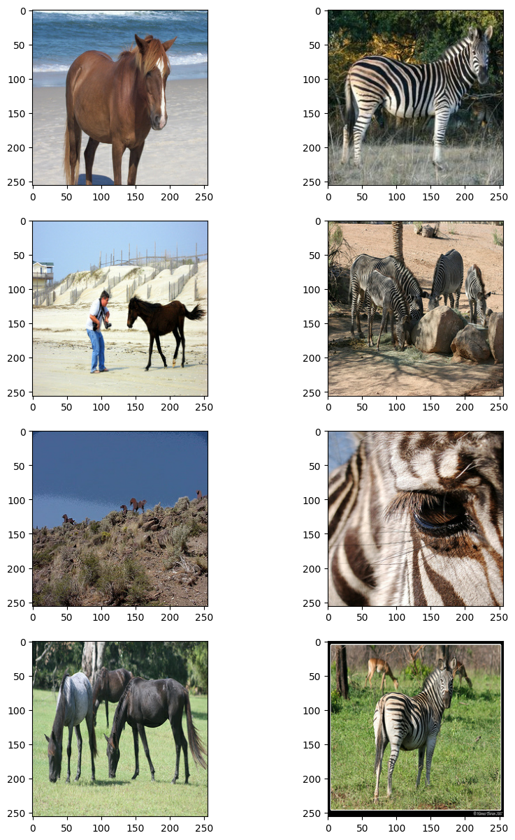
Graph Plotting by matplotlib.pyplot
We mainly use ax (array of axes)
import matplotlib.pyplot as plt _, ax = plt.subplots(4, 2, figsize=(10, 15)) for i, samples in enumerate(zip(train_horses.take(4), train_zebras.take(4))): horse = (((samples[0][0] * 127.5) + 127.5).numpy()).astype(np.uint8) zebra = (((samples[1][0] * 127.5) + 127.5).numpy()).astype(np.uint8) ax[i, 0].imshow(horse) ax[i, 1].imshow(zebra) plt.show()
Result:
ReflectionPadding2D
This is a built-in layer in pyTorch, but in tensorflow we need to built it manually:
class ReflectionPadding2D(layers.Layer): def __init__(self, padding=(1, 1), **kwargs): self.padding = tuple(padding) super(ReflectionPadding2D, self).__init__(**kwargs) def call(self, input_tensor, mask=None): padding_width, padding_height = self.padding # no padding for batch_size and channel axis padding_tensor = [ [0, 0], [padding_height, padding_height], [padding_width, padding_width], [0, 0], ] return tf.pad(input_tensor, padding_tensor, mode="REFLECT")
Residual Blocks
There are many version of residue blocks. In cycleGAN their blocks keep the number of filters and also the spatial dimension. In some other cases the middle Conv2D layer shrinks the filter depth and finally restored it for the addition operation in skip connection.
def residual_block( x, activation, kernel_initializer=kernel_init, kernel_size=(3, 3), strides=(1, 1), padding="valid", gamma_initializer=gamma_init, use_bias=False, ): dim = x.shape[-1] input_tensor = x x = ReflectionPadding2D()(input_tensor) x = layers.Conv2D( dim, kernel_size, strides=strides, kernel_initializer=kernel_initializer, padding=padding, use_bias=use_bias, )(x) x = tfa.layers.InstanceNormalization(gamma_initializer=gamma_initializer)(x) x = activation(x) x = ReflectionPadding2D()(x) x = layers.Conv2D( dim, kernel_size, strides=strides, kernel_initializer=kernel_initializer, padding=padding, use_bias=use_bias, )(x) x = tfa.layers.InstanceNormalization(gamma_initializer=gamma_initializer)(x) x = layers.add([input_tensor, x]) return x
Though the kenrnel_size is (3,3), but there will be a ReflectionPadding2D and therefore the finally the width
remains unchanged ( comes from padding), and so does the height.
Model.compile() and Model.train_step()
In GANs most of the last training step must be implemented manually. We record the one in cycleGAN for reference. The technique will apply to all other custom training.
Note the analogy with PyTorch's .backward() and .step().
class CycleGan(keras.Model): def __init__( self, generator_G, generator_F, discriminator_X, discriminator_Y, lambda_cycle=10.0, lambda_identity=0.5, ): super(CycleGan, self).__init__() self.gen_G = generator_G self.gen_F = generator_F self.disc_X = discriminator_X self.disc_Y = discriminator_Y self.lambda_cycle = lambda_cycle self.lambda_identity = lambda_identity def compile( self, gen_G_optimizer, gen_F_optimizer, disc_X_optimizer, disc_Y_optimizer, gen_loss_fn, disc_loss_fn, ): super(CycleGan, self).compile() self.gen_G_optimizer = gen_G_optimizer self.gen_F_optimizer = gen_F_optimizer self.disc_X_optimizer = disc_X_optimizer self.disc_Y_optimizer = disc_Y_optimizer self.bv = gen_loss_fn self.discriminator_loss_fn = disc_loss_fn self.cycle_loss_fn = keras.losses.MeanAbsoluteError() self.identity_loss_fn = keras.losses.MeanAbsoluteError() def train_step(self, batch_data): # x is Horse and y is zebra real_x, real_y = batch_data # For CycleGAN, we need to calculate different # kinds of losses for the generators and discriminators. # We will perform the following steps here: # # 1. Pass real images through the generators and get the generated images # 2. Pass the generated images back to the generators to check if we # we can predict the original image from the generated image. # 3. Do an identity mapping of the real images using the generators. # 4. Pass the generated images in 1) to the corresponding discriminators. # 5. Calculate the generators total loss (adverserial + cycle + identity) # 6. Calculate the discriminators loss # 7. Update the weights of the generators # 8. Update the weights of the discriminators # 9. Return the losses in a dictionary with tf.GradientTape(persistent=True) as tape: # Horse to fake zebra fake_y = self.gen_G(real_x, training=True) # Zebra to fake horse -> y2x fake_x = self.gen_F(real_y, training=True) # Cycle (Horse to fake zebra to fake horse): x -> y -> x cycled_x = self.gen_F(fake_y, training=True) # Cycle (Zebra to fake horse to fake zebra) y -> x -> y cycled_y = self.gen_G(fake_x, training=True) # Identity mapping # expect/hope that G|_{zebras} = id and F|_{horses} = idm # i.e., almost no change same_x = self.gen_F(real_x, training=True) same_y = self.gen_G(real_y, training=True) # Discriminator output disc_real_x = self.disc_X(real_x, training=True) disc_fake_x = self.disc_X(fake_x, training=True) disc_real_y = self.disc_Y(real_y, training=True) disc_fake_y = self.disc_Y(fake_y, training=True) # Generator adverserial loss gen_G_loss = self.generator_loss_fn(disc_fake_y) gen_F_loss = self.generator_loss_fn(disc_fake_x) # Generator cycle loss cycle_loss_G = self.cycle_loss_fn(real_y, cycled_y) * self.lambda_cycle cycle_loss_F = self.cycle_loss_fn(real_x, cycled_x) * self.lambda_cycle # Generator identity loss id_loss_G = ( self.identity_loss_fn(real_y, same_y) * self.lambda_cycle * self.lambda_identity ) id_loss_F = ( self.identity_loss_fn(real_x, same_x) * self.lambda_cycle * self.lambda_identity ) # Total generator loss total_loss_G = gen_G_loss + cycle_loss_G + id_loss_G total_loss_F = gen_F_loss + cycle_loss_F + id_loss_F # Discriminator loss disc_X_loss = self.discriminator_loss_fn(disc_real_x, disc_fake_x) disc_Y_loss = self.discriminator_loss_fn(disc_real_y, disc_fake_y) # Get the gradients for the generators # loss.backward() as in pyTorch grads_G = tape.gradient(total_loss_G, self.gen_G.trainable_variables) grads_F = tape.gradient(total_loss_F, self.gen_F.trainable_variables) # Get the gradients for the discriminators disc_X_grads = tape.gradient(disc_X_loss, self.disc_X.trainable_variables) disc_Y_grads = tape.gradient(disc_Y_loss, self.disc_Y.trainable_variables) # Update the weights of the generators # optimizer.step() as in pyTorch self.gen_G_optimizer.apply_gradients( zip(grads_G, self.gen_G.trainable_variables) ) self.gen_F_optimizer.apply_gradients( zip(grads_F, self.gen_F.trainable_variables) ) # Update the weights of the discriminators self.disc_X_optimizer.apply_gradients( zip(disc_X_grads, self.disc_X.trainable_variables) ) self.disc_Y_optimizer.apply_gradients( zip(disc_Y_grads, self.disc_Y.trainable_variables) ) # Conclusion: the only difference to pytorch is that we need to # wrap the calculation of loss to get the calculation graph # i.e., wrap the stuff whose weight needs to be updated. # which usually starts from the beginning of getting batch_data return { "G_loss": total_loss_G, "F_loss": total_loss_F, "D_X_loss": disc_X_loss, "D_Y_loss": disc_Y_loss, }
Monitor
class GANMonitor(keras.callbacks.Callback): """A callback to generate and save images after each epoch""" def __init__(self, num_img=4): self.num_img = num_img def on_epoch_end(self, epoch, logs=None): _, ax = plt.subplots(4, 2, figsize=(12, 12)) for i, img in enumerate(test_horses.take(self.num_img)): prediction = self.model.gen_G(img)[0].numpy() prediction = (prediction * 127.5 + 127.5).astype(np.uint8) img = (img[0] * 127.5 + 127.5).numpy().astype(np.uint8) ax[i, 0].imshow(img) ax[i, 1].imshow(prediction) ax[i, 0].set_title("Input image") ax[i, 1].set_title("Translated image") ax[i, 0].axis("off") ax[i, 1].axis("off") prediction = keras.preprocessing.image.array_to_img(prediction) prediction.save( "generated_img_{i}_{epoch}.png".format(i=i, epoch=epoch + 1) ) plt.show() plt.close()
Start the Training Process
Our gen_G and gen_F only need optimizer, we calculate the loss on our own. We also pass tensorflow built-in loss functions for convenience (which will turns out to be one of the summands in our total loss).
# Loss function for evaluating adversarial loss adv_loss_fn = keras.losses.MeanSquaredError() # Define the loss function for the generators def generator_loss_fn(fake): fake_loss = adv_loss_fn(tf.ones_like(fake), fake) return fake_loss # Define the loss function for the discriminators def discriminator_loss_fn(real, fake): real_loss = adv_loss_fn(tf.ones_like(real), real) fake_loss = adv_loss_fn(tf.zeros_like(fake), fake) return (real_loss + fake_loss) * 0.5 # Create cycle gan model cycle_gan_model = CycleGan( generator_G=gen_G, generator_F=gen_F, discriminator_X=disc_X, discriminator_Y=disc_Y ) # Compile the model cycle_gan_model.compile( gen_G_optimizer=keras.optimizers.Adam(learning_rate=2e-4, beta_1=0.5), gen_F_optimizer=keras.optimizers.Adam(learning_rate=2e-4, beta_1=0.5), disc_X_optimizer=keras.optimizers.Adam(learning_rate=2e-4, beta_1=0.5), disc_Y_optimizer=keras.optimizers.Adam(learning_rate=2e-4, beta_1=0.5), gen_loss_fn=generator_loss_fn, disc_loss_fn=discriminator_loss_fn, ) # Callbacks plotter = GANMonitor() checkpoint_filepath = "./model_checkpoints/cyclegan_checkpoints.{epoch:03d}" model_checkpoint_callback = keras.callbacks.ModelCheckpoint( filepath=checkpoint_filepath ) # Here we will train the model for just one epoch as each epoch takes around # 7 minutes on a single P100 backed machine. cycle_gan_model.fit( tf.data.Dataset.zip((train_horses, train_zebras)), epochs=1, callbacks=[plotter, model_checkpoint_callback], )